在正式剖析 Autograd Engine 之前, 有必要先花一点时间把多元微积分里 “导数” 与 “偏导数” 这两个概念重新捋一遍, 毕竟我发现自己又在这块儿犯迷糊了. 严格而系统的论述请参考 陶 Analysis II 6: 多元微分学, 下文仅为个人的非严谨提醒, 旨在把最关键的直觉再钉牢一点.
对于函数 $f: \mathrm{R}^n \to \mathrm{R}^m$, $f$ 在点 $x_0$ 处关于变量 $x_j$ 的偏导数记作 $\frac{\partial f}{\partial x_j}(x_0) \in \mathrm{R}^m$. 偏导数可以通过这样的方式来得到: 固定除了 $x_j$ 以外的所有变量, 然后把函数看作关于 $x_j$ 的单变量函数, 进而求其导数. 如果我们把 $f$ 写成 $f = (f_1, f_2, \cdots, f_m)$, 那么 $\frac{\partial f_i}{\partial x_j}(x_0) \in \mathrm{R}$ 且有:
\[\frac{\partial f}{\partial x_j}(x_0) = \left(\frac{\partial f_1}{\partial x_j}(x_0), \cdots, \frac{\partial f_m}{\partial x_j}(x_0)\right)\]若 $f$ 在点 $x_0$ 处可微, 那么 $f$ 在点 $x_0$ 处导数 $f’(x_0)$ 是个线性变换(不是一个具体的值/向量)! 对应着一个 $\mathrm{R}^{m \times n}$ 矩阵, 不严谨地说:
\[f'(x_0) = \begin{pmatrix} \frac{\partial f_1}{\partial x_1}(x_0) & \cdots & \frac{\partial f_1}{\partial x_n}(x_0) \\ \vdots & \vdots & \vdots \\ \frac{\partial f_m}{\partial x_1}(x_0) & \cdots & \frac{\partial f_m}{\partial x_n}(x_0) \\ \end{pmatrix}\]有结论 $\frac{\partial f}{\partial x_j}(x_0) = f’(x_0) e_j$. 另有结论对于 $f \in \mathrm{R}^n \to \mathrm{R}^m, g: \mathrm{R}^m \to \mathrm{R}^p$, 那么:
\[(g \circ f)'(x_0) = g'(f(x_0))f'(x_0)\]别忘了这里 $f’(x_0)$ 是个线性映射, 对应着 $\mathrm{R}^{m \times n}$. 同样 $g’(f(x_0)) \in \mathrm{R}^{p \times m}$. 即 $(g \circ f)’(x_0) \in \mathrm{R}^{p \times n}$
现在来实战一下, 给定 $f(x_1, x_2) = (\log(x_1 x_2), \sin(x_2)), g(y_1, y_2) = y_1 y_2, z = g \circ f$, 求取 $\frac{\partial z}{\partial x_1}(x_0), \frac{\partial z}{\partial x_2}(x_0)$:
\[\begin{gather} \frac{\partial z}{\partial x_1}(x_0) = z'(x_0) e_1 \\ z'(x_0) = (g \circ f)'(x_0) = g'(f(x_0)) f'(x_0) \\ g'(f(x_0)) = \left( \frac{\partial g}{\partial y_1}(f(x_0)), \frac{\partial g}{\partial y_2}(f(x_0)) \right) = \left( y_2^v, y_1^v \right) \\ f'(x_0) = \begin{pmatrix} \frac{\partial f_1}{\partial x_1}(x_0) & \frac{\partial f_1}{\partial x_2}(x_0) \\ \frac{\partial f_2}{\partial x_1}(x_0) & \frac{\partial f_2}{\partial x_2}(x_0) \end{pmatrix} = \begin{pmatrix} \frac{1}{x_1^v} & \frac{1}{x_2^v} \\ 0 & \cos(x_2^v) \end{pmatrix} \\ z'(x_0) = \left( \frac{y_2^v}{x_1^v}, \frac{y_2^v}{x_2^v} + y_1^v \cos(x_2^v) \right) \\ \frac{\partial z}{\partial x_1}(x_0) = \frac{y_2^v}{x_1^v} \\ \frac{\partial z}{\partial x_2}(x_0) = \frac{y_2^v}{x_2^v} + y_1^v \cos(x_2^v) \end{gather}\]因此给定 $x_0 = (0.5, 0.75)$ 可得 $\left( \frac{\partial z}{\partial x_1}(x_0), \frac{\partial z}{\partial x_2}(x_0) \right) = (1.3633, 0.1912)$:
>>> x1 = 0.5; x2 = 0.75;
>>> y1 = math.log(x1 * x2); y2 = math.sin(x2)
>>> y2 / x1
1.3632775200466682
>>> y2 / x2 + math.cos(x2) * y1
0.19118983333660755
P.S. 如同在 再读 Gpipe, 前向传播, 后向传播 提到的, 这里 $y_2^v$ 表示具体的值, 不是参数; $x_0 = (x_1^v, x_2^v), f(x_0) = (y_1^v, y_2^v)$.
P.S. 我发现 AI 这块同学习以为常地喜欢用 $\frac{\partial f}{\partial x_j}$ 来表示在某点的偏导数 $\frac{\partial f}{\partial x_j}(x_0)$, 让我花了一段时间适应这种用法=
pytorch autograd
那么 pytorch 是怎么实现 autograd 的呢? 她会把 $z’(x_0) = g’(f(x_0)) f’(x_0)$ 这里用到的矩阵构造出来么?
>>> x = torch.tensor([0.5, 0.75], requires_grad=True)
>>> y = torch.log(x[0] * x[1]) * torch.sin(x[1])
>>> y.backward()
>>> x.grad
tensor([1.3633, 0.1912])
并不会, 正如 Going through the graph 提到的:
Every time PyTorch executes an operation, the autograd engine constructs the graph to be traversed backward. when PyTorch records the computational graph, the derivatives of the executed forward operations are added (Backward Nodes). Once the forward pass is done, the Jvp calculation starts but it never constructs the matrix. They take their primitive function inputs and outputs as parameters along with the gradient of the function outputs with respect to the final outputs. By repeatedly multiplying the resulting gradients by the next Jvp derivatives in the graph, the gradients up to the inputs will be generated following the chain rule.
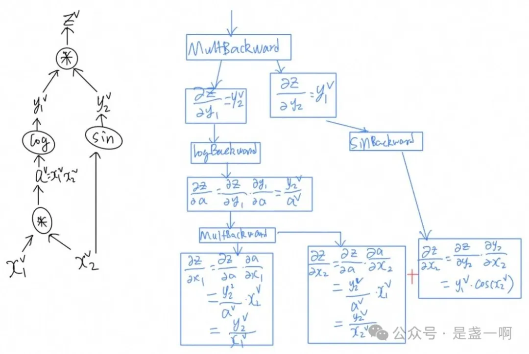
最让我惊奇的是 $\frac{\partial z}{\partial x_2}$ 的计算, 这个是由两个不同的来源产生的; 在 pytorch 中, 当两个不同的函数共享同一个输入时, 针对该输入的关于输出的梯度会被累加起来; 在所有路径的梯度没有全部聚合完成之前, 使用该梯度进行的计算是无法继续的.
那么这里梯度被累加总是正确的么? 当然是了!
\[\begin{gather} L = F(z_1, z_2): \mathrm{R}^2 \to \mathrm{R} \\ G(x) = (G_1(x), G_2(x)): \mathrm{R} \to \mathrm{R}^2 \\ L(x) = (F \circ G) (x): \mathrm{R} \to \mathrm{R} \\ L'(x_0) = F'(G(x_0)) G'(x_0) \\ F'(G(x_0)) = \left( \frac{\partial F}{\partial z_1}(G(x_0)) , \frac{\partial F}{\partial z_2}(G(x_0)) \right) \\ G'(x_0) = \begin{pmatrix} \frac{\partial G_1}{\partial x} (x_0) \\ \frac{\partial G_2}{\partial x} (x_0) \end{pmatrix} \\ L'(x_0) = \frac{\partial F}{\partial z_1}(G(x_0)) \frac{\partial G_1}{\partial x} (x_0) + \frac{\partial F}{\partial z_2}(G(x_0)) \frac{\partial G_2}{\partial x} (x_0) \end{gather}\]即同一个变量 $x$ 同时影响 $z_1$ 和 $z_2$, 并通过不同路径影响 $L$. Path A: $x \to z_1 \to L$, Path B: $x \to z_2 \to L$. 这里 $\frac{\partial F}{\partial z_1}(G(x_0)) \frac{\partial G_1}{\partial x} (x_0)$ 对应 PathA backward 求取出的梯度, $\frac{\partial F}{\partial z_2}(G(x_0)) \frac{\partial G_2}{\partial x} (x_0)$ 对应 PathB backward 求取出的梯度. 对同一个变量的梯度贡献, 来自每条路径的结果需要 相加.