PaperReading: Nanoflow

在 CPU 中, 当我们只调度一个执行流给 CPU 时, 如果 CPU 在执行某些指令时遇到了阻塞, 比如在执行 io 指令时, 此时整个 CPU 将处于闲置状态, 其会等待 io 指令执行完成才开始处理下一条指令. 这造成了浪费, 而我们看不得浪费. 为此引入了超线程技术, 允许应用将两个执行流调度到一个 CPU 上, 这样当 CPU 执行一条执行流阻塞时会切换执行下一个执行流. 与此同时乱序执行, 多流水线等各种技术都引入进来, 使得即使只调度了一个执行流给 CPU, CPU 也会想尽办法在执行指令 x 阻塞时调度其他不依赖 x 的指令执行. 而 GPU 也面临着同样的问题, nanoflow 就是尝试在软件层面解决这些问题. 在模型推理时, 当前推理框架会将如下图所示执行流调度到 gpu 中:

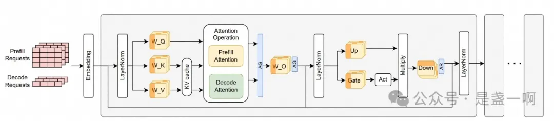
在 gpu 执行这条执行流时, 当忙着执行其中一个 operation 时, 比如这个 AllGather, 此时 AG operation 只会使用 network resource, 这导致 GPU compute/memory resource 都处于闲置状态, 但由于执行流中 operation 天然的依赖关系, GPU 无法调度执行其他可以用到 compute/memory resource 的 operation. 解决思路也很直观, 就像 CPU 超线程一样, 我们一次调度多个执行流给 gpu, 多个执行流中 operation 互相之间可没有依赖关系. 当然也不能无脑调度多个执行流, 就像 CPU 超线程中经常会遇到由于资源争抢, 调度到同一 CPU 的两个执行流执行速度都会变慢. 为此 nanoflow 为单个 GPU 精心设计了一条执行流 v1:

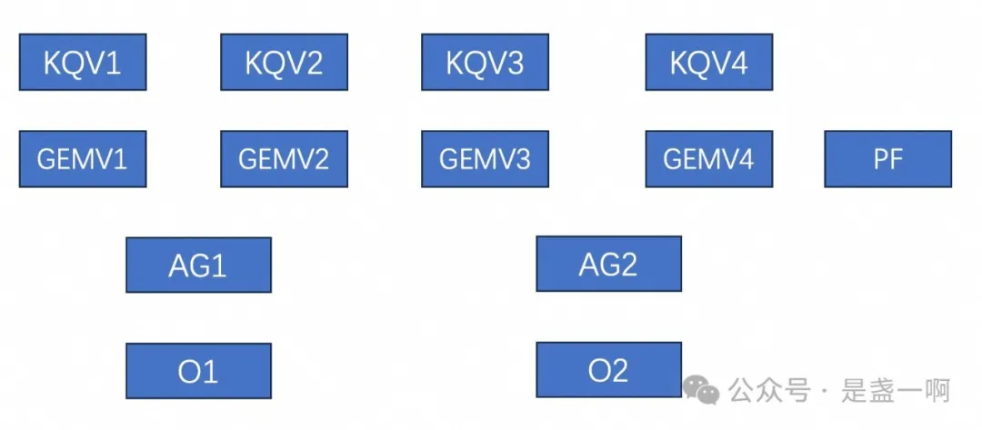
此时 GPU 输入是一个 batch, 其内包含 prefill req/decode req, nanoflow 会将其切分为 4 个 nanobatch, decode req 会平均分配到 4 个 nanobatch 中, 之后将第 i 个 nanobatch 下发给第 i 个 KQV 对应的执行流. 这里 KQV 用于计算 K, Q, V; GEMV 用于计算 Decode attention, PF 用于计算 prefill attention. KQVi 在完成计算之后会将其中的 decode req 分发给对应的 GEMVi 计算 decode attention, 将 prefill req 下发给 PF 计算 prefill attention. nanoflow 将节点内多个 GPU 组成了一个 tp group, AG, AllGather 算子用来汇聚其他 GPU 的计算结果. O1, O2 对应着 O-projection, 这里 O2 负责处理所有 decode req, O1 负责处理 prefill req. 这导致了 O2 必须需要等待 AG2, nanoflow 不喜欢等待. 为此其将执行流调整如下, 执行流 v2:

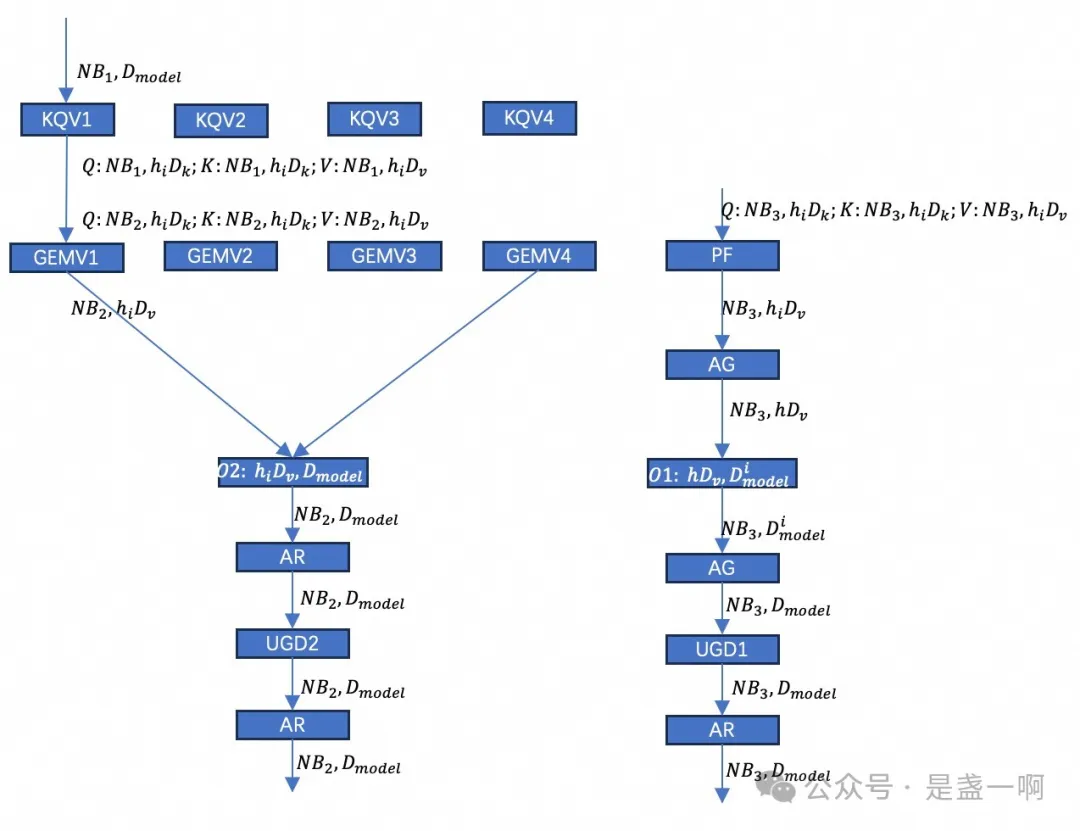
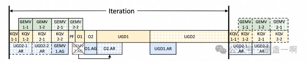
图中 $h_i, D^i_{model}$ 表示 tp group 第 i 个分片. 如上执行流最理想执行情况是, 如下所示此时 resource overlap 达到了最佳, 确保 compute/network/memory resource 没有一丝偷闲的机会:

GPU 实现

在完成如上流水线设计之后, 接下来一个问题就是对于一个给定的模型, 如何确定流水线中每个操作输入 nanobatch 的大小, 以及每个操作占用多少资源. 毕竟稍有不慎, 就会像 CPU 超线程那样造成了资源争抢两败俱伤. nanoflow 这里解法见 5.5 Automatic parameter search.

在完成参数确定之后, 我们便知道了每个 kernel operation 应该用多少资源, nanoflow 这里好像是通过 multi-stream 以及在启动 kernel 中配置 thread block 数目来表示 kernel 应该使用多少资源, 因为看到其在 attention kernel 那里提到过: 假设目前 attention kernel 是面向 M thread block 设计的, 但是在启动时由于资源限制只能为其分配 N thread block, 此时 , each thread block will sequentially execute the workload that was originally ssigned to $\left \lceil M/N \right \rceil$ thread blocks. 看样子 nanoflow 没有使用类似 libsmctrl 这类黑科技. 后面这块需要进一步通过代码确认下. 另外这里应用了 GPU 黑盒特性, The key insight that supports execution unit scheduling is the non-linearity of GPU resource utilization, 以 network operation 举例, with only 35 SMs out of 108 SMs (32%), network kernels can achieve up to 92% peak performance. 也就是说并不需要为 network kernel 分配所有 SM 才能打满 network bandwidth. 这种数据只能 case-by-case 测试出来了.

CPU 实现

即使是在 CPU 任务处理上, nanoflow 会尽最大努力不让 GPU 闲着, 这主要体现在:

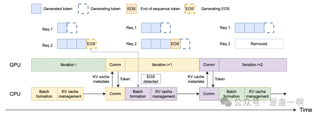
5.3 Top-level scheduling, 全异步化, 尽最大可能与 gpu overlap.

async kvcache offload. nanoflow 支持 prompt cache, 会在请求结束时将请求 kvcache 卸载保存到 SSD 上, 并采用 LRU 策略管理. 考虑到将 kvcache offload ssd 对于 gpu 来说是个 memory bound 操作, nanoflow 会在下一次迭代 UGD 期间调度 offload 任务, 来尽可能 overlap. 为了提升 offload 吞吐, 在 offload 时, nanoflow 会先将分布在各地的 kvcache page 聚合到一段连续空间中, 之后将这段连续空间中的内容卸载到 ssd. 在从 ssd 中加载 kvcache 到 gpu 中时也具有类似的过程. 另外这里 nanoflow 也考虑了 numa 亲和.

杂项

接着上面的实现框架, 再过一遍论文, 记录一些有意思的点.

2.1 节这个 up, gate 来自 GLU Variants Improve Transformer, 对应实现:

class MLP(nn.Module):
  def forward(self, hidden_states):
    # 继续用 '从 transformer 到 FlashAttention 再到 PagedAttention(1)' 的语言
    # 来描述这里各个矩阵维度, 这里 MLP 对应着 transformer FFN:
    # hidden_states, 类似于 x. (n_0, d_model).
    # gate_proj, 类似于 W_1, (d_model, 2/3 W_ff)
    # up_proj, 类似于 W_1, (d_model, 2/3 W_ff)
    # down_proj, 类似于 W_2, (2/3 W_ff, d_model)
    gate = F.silu(self.gate_proj(hidden_states))
    up = self.up_proj(hidden_states)
    return self.down_proj(gate * up)

In total, two AGs and one AR operation are needed for NanoFlow’s inference workflow. 但实际上, 就像 Megatron 中一样, 只需要 2 AR 就可以的. 但我这里算了下, 实际上这里 AR 通信时间与数据量与 2AG 是一样的.

NanoFlow’s batch scheduler introduces discrete batching, which chooses the dense batch size $B_{dense}$ among a few high-performance batch sizes instead of arbitrary ones to maximize the efficiency of dense operations.

我理解这里先通过 offline profile 方式测出一组 high-performance batch sizes, 之后在线上接受请求中, 会从这些 batch size 选择一个, 比如现在最优 batch size 为 2, 4, 8; 现在到来 9 个请求, 则会先下发 8 个请求进行一次 iteration, 在这个 iteration 结束之后再下发剩下的那 1 个请求. dynamically chooses the system batch size according to the system load 意味着这 9 个请求也可能会拆分为 4 + 2 + 2 + 1 的形式.

参见上面流水线 v2, 我本来以为在 PF 之前也会加一个 batch scheduler 确保 PF 输入 batch size $NB_3$ 是个最优 batch. 但现在看来好像没必要, global batch scheduler 会确保 nanobatch size $NB_1$ 以及其内 prefill/decode 请求比例, 从而确保 $NB_2, NB_3$ 都是最优的.

batch scheduler adopts tensor parallelism within a node and simply feeds the entire batch into all GPUs instead of micro-batching. 也就是 nanoflow 不考虑 pp. feeds the entire batch into all GPUs 应该意味着其像 Megatron 一样 layernorm 这些层会重复计算, 每个 gpu 上做相同的计算.

Peak memory estimation 这里, ‘the average decode length’ 是 $d$ 么? 如果是 d 的话都没必要为每一个 on-fly 请求追踪当前 decoded token 个数了, 直接维护个 on-fly 请求个数 $n, n * d$ 就是 total decode length 了. 所以这里 ‘the average decode length’ 应该不是 $d$, 而是类似一个移动平均值这样的东西. 需要结合源码确认下.

calculates the highest future memory usage, 假设我们上面预测出来的 total decode length 是 T, 那这里是通过 T token 还是像公式 (5) 一样使用 T/2 来预估 kvcache 占用? 需要结合源码确认下.

建模

nanoflow 第 3 章对模型推理过程进行了建模, 分析了在一次 iteration, 即 where a batch of user requests are being processed by all the transformer layers, 花费在 memory, compute, network 资源上的时间. 我这里挑一些一开始我没读明白的点记一下:

$2 B_{Dense} P_{Model}$ 的由来, 由 dense operation 的定义可知这里都是 GEMM, 且矩阵乘法双方形状是 $(B_{Dense}, N_w) \times (N_w, K_w)$, 不同的 dense op 对应着不同的 $N_w, K_w$; 一次 iteration 所有 dense operation 运算总和为 $2 B_{Dense} \sum N_w K_w \approx 2 B_{Dense} P_{Model}$. 这里 $B_{Dense}$ 就是本次 iteration batch 中包含的输入 token 数目.

公式 (2) $B_{Dense} = \frac{B_{req}(p + d)}{d+1}$ 的由来, 对于一个特定的请求而言, 其需要 1 次 prefill iteration + d 次 decode iteration; 即其有 $\frac{1}{d+1}$ 的概率处于 prefill iteration 以及 $\frac{d}{d+1}$ 的概率处于 decode. 对于一个特定 iteration 而言, 其包含了 $B_{req}$ 请求, 其中大概 $\frac{1}{d+1} B_{req}$ 的请求处于 prefill, $\frac{d}{d+1} B_{req}$ 的请求处于 decode. 即可得公式 (2).

As each request requires a KV-cache with the capacity of $p + \frac{d}{2}$ tokens on average, 我的理解是对于一个特定请求, 其初始需要 p token, 最终需要 p + d; 但这个不是上来就需要为 p + d token 申请 kv cache, 而是随着 iteration 迭代逐步增加的, 所以平均了一下, 需要 $p + \frac{d}{2}$.

Network 这里公式推导应该是: 这里 p 表示 tp group 中 gpu 数目, B 表示带宽. 很明显在 nanoflow 这里 $p - 1 = p$~

\[\underbrace{\frac{p-1}{B} \frac{n_i d_{model}}{p}}_{AG} + \underbrace{\frac{p-1}{B} \frac{n_i d_{model}}{p}}_{AG} + \underbrace{2 \frac{p-1}{B} \frac{n_i d_{model}}{p}}_{AR}\]

这里 $n_i d_{model}$ 是矩阵中元素个数, 换算为字节的话, $n_i d_{model} D_{type}$. 这里 $n_i$ 就是 $B_{Dense}$, 我只是个人习惯, 接着用了上面推导 2AG = AR 时的符号.

我个人认为接下来要研究的就是如何在 overlap 前提下尽量让 kernel operation 之间互不影响了

However, due to inevitable kernel interference, NanoFlow still has a gap between optimal compute usage.

参考

再读 Gpipe, 前向传播, 后向传播
从 transformer 到 FlashAttention 再到 PagedAttention(1)
Ring All-reduce的数学性质
NanoFlow P.S. 微信公众号会给图片加上水印, 这实非我愿!

GPU 实现

CPU 实现

杂项

建模

Next

参考

CATALOG